Machine learning

Suppose that you’re looking for a new apartment. You speak to friends and family, and do some online searches for apartments in the city. You notice that apartments in different areas are priced differently. Here are some of your observations from all your research:

• A one-bedroom apartment in the city center (close to work) costs $5,000 per month.
• A two-bedroom apartment in the city center costs $7,000 per month.
• A one-bedroom apartment in the city center with a garage costs $6,000 per month.
• A one-bedroom apartment outside the city center, where you will need to commute to work, costs $3,000 per month.
• A two-bedroom apartment outside the city center costs $4,500 per month.
• A one-bedroom apartment outside the city center with a garage costs $3,800 per month.

You notice some patterns. Apartments in the city center are most expensive and are usually between $5,000 and $7,000 per month. Apartments outside the city are cheaper. Increasing the number of rooms adds between $1,500 and $2,000 per month, and access to a garage adds between $800 and $1,000 per month.

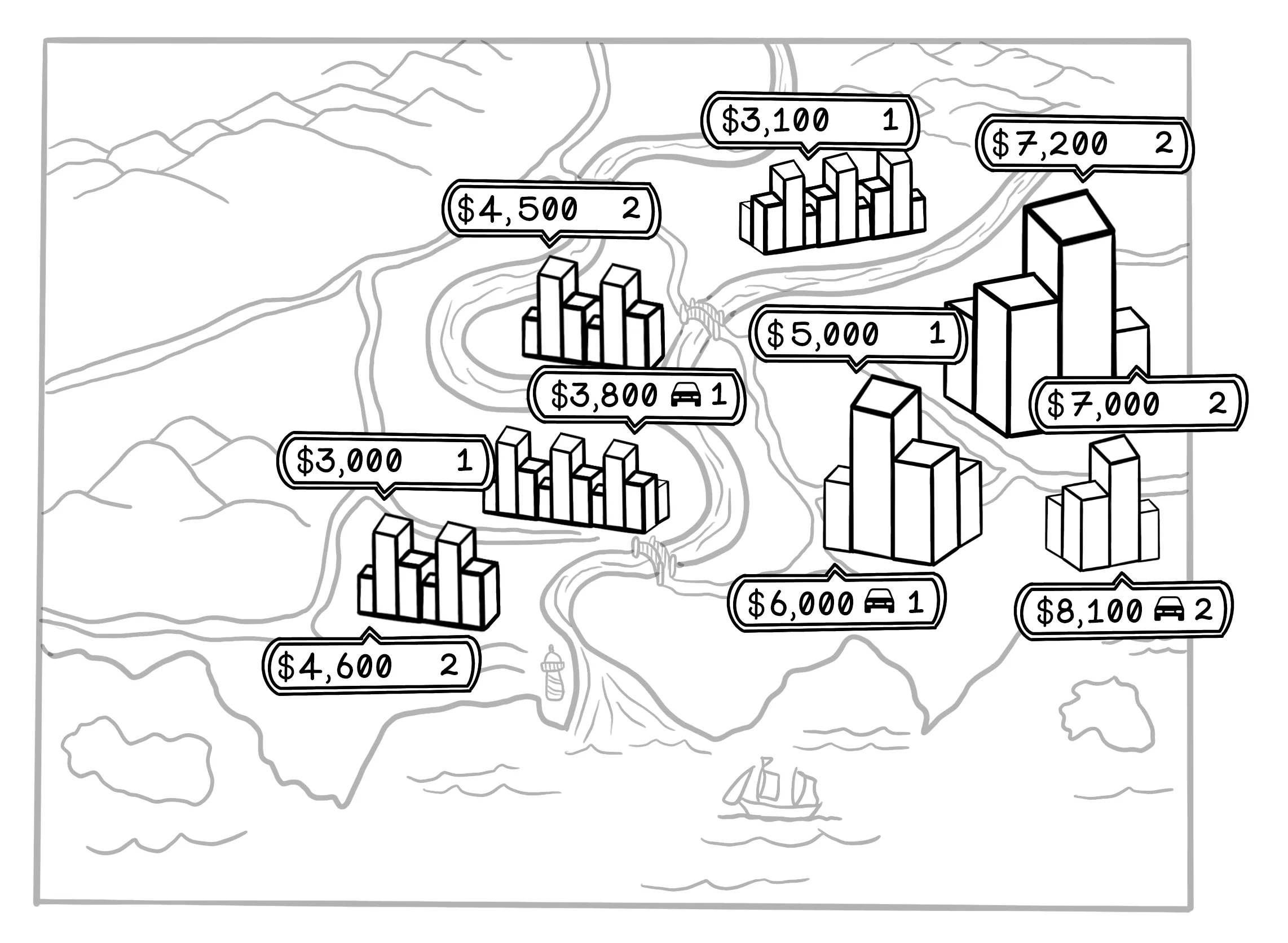
This example shows how we use data to find patterns and make decisions. If you encounter a two-bedroom apartment in the city center with a garage, it’s reasonable to assume that the price would be approximately $8,000 per month.

Machine learning aims to find patterns in data for useful applications in the real world. We could spot the pattern in this small dataset, but machine learning spots them for us in large, complex datasets.

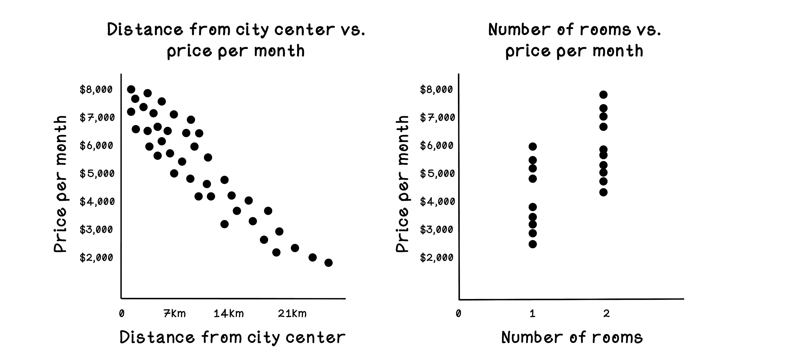
Notice that there are more dots closer to the city center and that there is a clear pattern related to price per month: the price gradually drops as distance to the city center increases. There is also a pattern in the price per month related to the number of rooms; the gap between the bottom cluster of dots and the top cluster shows that the price jumps significantly. We could naïvely assume that this effect may be related to the distance from the city center. Machine learning algorithms can help us validate or invalidate this assumption. We dive into how this process works throughout this chapter.

Choosing an algorithm to use is based largely on two factors: the question that is being asked and the nature of the data that is available. If the question is to make a prediction about the price of a diamond with a specific carat weight, regression algorithms can be - useful. The algorithm choice also depends on the number of features in the dataset and the relationships among those features. If the data has many dimensions (there are many features to consider to make a prediction), we can consider several algorithms and approaches.

Regression means predicting a continuous value, such as the Price or Carat of the diamond. Continuous means that the values can be any number in a range. The price of $2,271, for example, is a continuous value between 0 and the maximum price of any diamond that regression can help predict.

Linear regression is one of the simplest machine learning algorithms: it finds relationships between two variables and allows us to predict one variable given the other. An example is predicting the price of a diamond based on its carat value. By looking at many examples of known diamonds, including their Price and Carat values, we can teach a model the relationship and ask it to make predictions.

Diamond	Carat	Price
1	0.71 ct	$1,643
2	0.70 ct	$2,241
3	0.61 ct	$931
4	0.30 ct	$1,013
5	0.24 ct	$419
6	2.00 ct	$12,576

Let’s start trying to find a trend in the data and attempt to make some predictions. For exploring linear regression, the question we’re asking is “Is there a correlation between the carats of a diamond and its price, and if there is, can we make accurate predictions?”

We start by isolating the Carat and Price features and plotting the data on a graph. Because we want to find the price based on Carat value, we will treat carats as x and price as y. Why did we choose this approach?

• Carat as the independent variable (x) — An independent variable is one that is changed in an experiment to determine the effect on a dependent variable. In this example, the value for carats will be adjusted to determine the price of a diamond with that value.

• Price as the dependent variable (y) — A dependent variable is one that is being tested. It is affected by the independent variable and changes based on the independent variable value changes. In our example, we are interested in the price given a specific carat value.

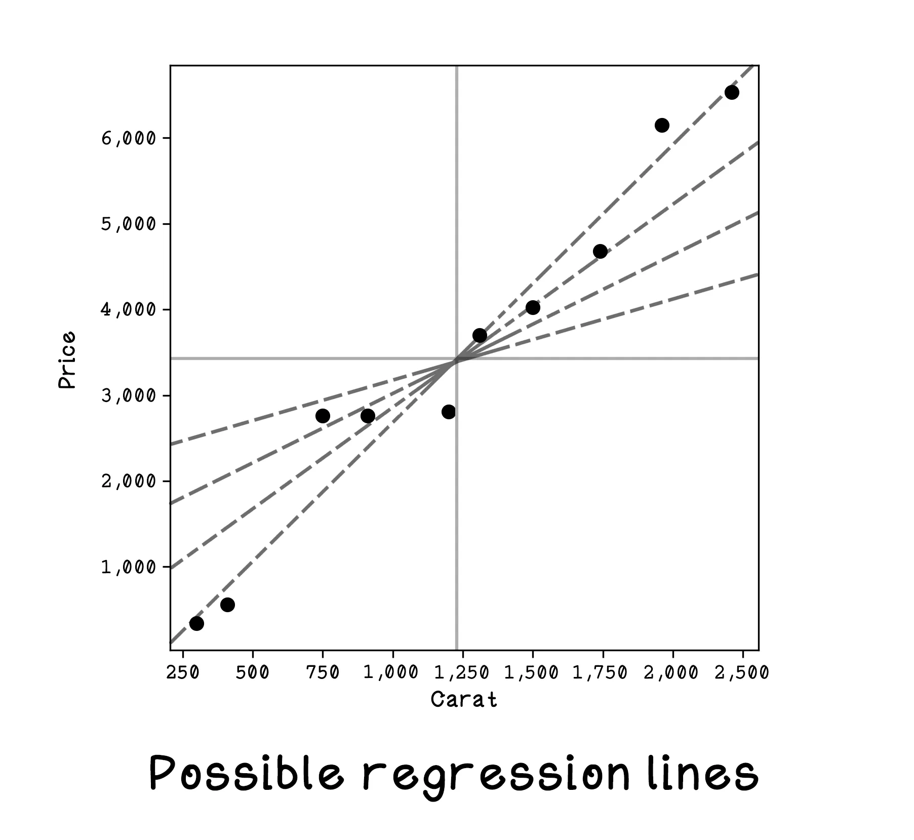
Linear regression will always find a straight line that fits the data to minimize distance among points overall. Understanding the equation for a line is important because we will be learning how to find the values for the variables that describe a line.

A straight line is represented by the equation y = c + mx:

• y: The dependent variable
• x: The independent variable
• m: The slope of the line
• c: The y-value where the line intercepts the y axis

Play with the learning rate and see how the linear regression model fits to the diamond carat-price data.